我们正在向新域名迁移,3秒后自动跳转
We are migrating to new domain, will redirect in 3 seconds
jackwish.net -----> zhenhuaw.me
Boost Quantization Inference Performance
This tech report was originally written for TVM community to share the techniques and experiences of optimizing quantization inference performance on ARM devices by using TVM. We opened pull request to the community, but the community seems not ready to accept the report because the code has not been open sourced yet. As I have left the team, the open source is out of my ability. Anyway, I’d like to share the work as it is really impressive, it doesn’t matter whether the report is placed in the official community website.
Background
For years, deep learning has been one of the core technologies across data centers and edge devices. AliOS, with the vision of driving all intelligent things, keeps putting efforts in functionality enabling and performance tuning for edge devices based on TVM. Some of the key results have been presented at TVM Shanghai Meetup (slides) and TVM Conference 2019 (slides).
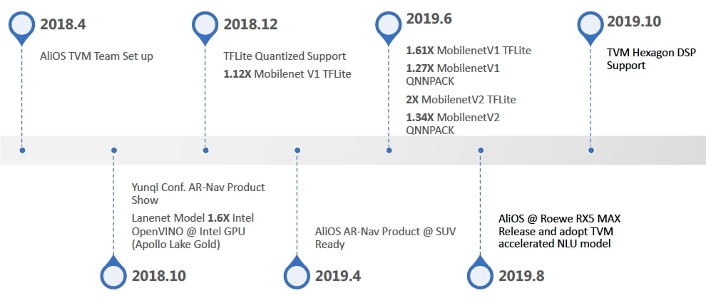 Figure 1: Milestones of AliOS TVM Team.
As shown in Figure 1, we enabled TensorFlow/TFLite flavored quantization support in late 2018. Figure 2 demonstrates the workflow, where the quantization (converting model from float32 to uint8) is handled by TensorFlow Quantization-aware Training and TensorFlow Lite Model Converter, and TVM imports quantized TensorFlow Lite models (*.tflite), builds and deploys.
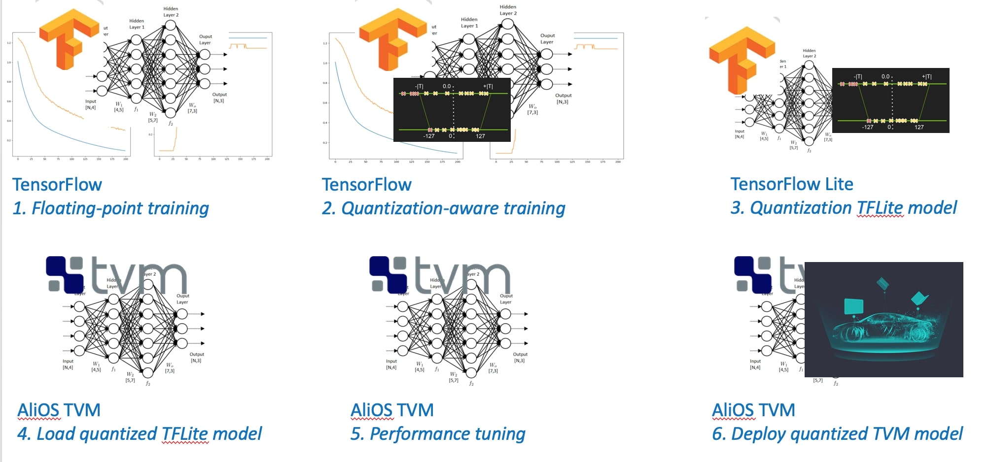 Figure 2: Workflow of TFLite-flavored Quantization on TVM
This approach offloads quantization accuracy issue to existing product-ready software stack, and centralizes development resources to inference performance. The TFLite frontend has been open sourced and the workflow approach has been adopted by the community.
However, as in Figure 1, the initial optimization (Dec. 2018) for quantization received 12% performance advantage over TFLite only.
As inference latency is very important, we focused on performance tuning for ARM CPU during the first half of 2019. This post shares related techniques and experiences.
Convolution Optimization
The techniques employed in our optimization can be roughly categorized into three, and will be discussed one by one in this section.
Tensorize Micro Kernel
Careful analysis of the assembly of initial optimization shows that the existing schedule algorithm can hardly generate efficient code for quantization. The observations are summarized into three problems:
-
The loading and computing are sometimes poorly-vectorized due to convolution computation pattern.
-
The register utilization is not efficient enough.
-
The data bandwidth between registers and memory is poorly-managed.
Problem 1 and 2 root from the schedule primitives of TVM which are high level abstracted. Problem 3 is due to limitation of reductions are only allowed at the top level of compute, in which way int32 memory access cannot be eliminated by fusing compute stages.
Tensorize is the technique for such scenarios, with which we can manipulate a fine-grain micro kernel. In one word, Tensorize identifies a compute pattern and replaces it with a customized computation, which can be either a micro kernel or hardware intrinsic. For example, the core loop of tiled matrix multiplication in Figure 3 can be replaced by gemm_1x4().
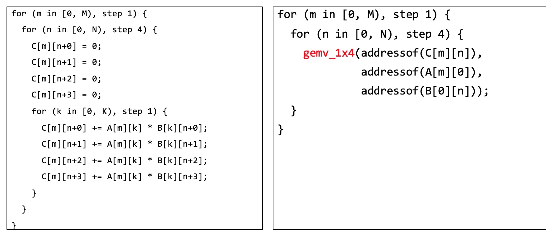 Figure 3: A Tensorize Example of Matrix Multiplication.
The compute replacement ability enabled by Tensorize resolves Problem 1 and 2. For Problem 3, regarding schedule limitations, we employed a trick. Since the pattern of original compute and customized one are only to match and replace computation in Tensorize mechanism, it is unnecessary to be the semantic of the original compute. In practice, we build a dummy computation naming fake_conv, which aims to capture the memory buffer only. The original compute semantic is handled by micro kernel itself. The trick is something like dummy functions of shared libraries only to satisfy dynamic linking, Android NDK libraries for example.
With Tensorize and optimized novel schedule algothrim, the problems mentioned in the beginning of this section are no longer barriers of performance. Besides, some other optimizations such as software pipeline have also been used.
Switch to NHWC Data Layout
As we know, data layout of convolution neural network (CNN) includes NCHW, NHWC, etc. among which TVM takes NCHW for CPU.
Though with Tensorize enabled, performance didn’t improve much as expected. As the micro kernel controls every instructions of the core loop, we pay attention to coarse-grain computation.
We investigated pointwise convolution which is equal to matrix multiplication in computation. Profiling tool reports high L1 cache miss rate 40%, while only 1% of QNNPACK (a high-performance kernel library released by PyTorch project), as Figure 4. But why?
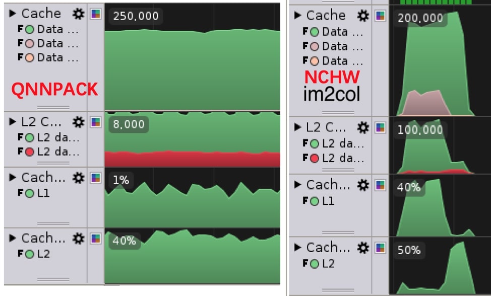 Figure 4: Cache Miss of QNNPACK and our NCHW Implementation.
As pointwise convolution is equivalent to the computation of matrix multiplication, the schedule algothrim tiles computation into $8 \times 8$ block. The tiled block is tensorized by micro kernel gemm_8x8(), which walks over reduction dimension by stepping 8, highlighted in Figure 5 (drawing \(4 \times 4\) for simplicity).
Now looking into the detail. In Figure 5, inside and outside means the cache behavior of the block. Also note that, cache behavior of output and filter can be ignored because:
-
The tensorized micro kernel stores data onto output only once.
-
The filter can be transformed into any layout offline with the help of AlterOpLayout.
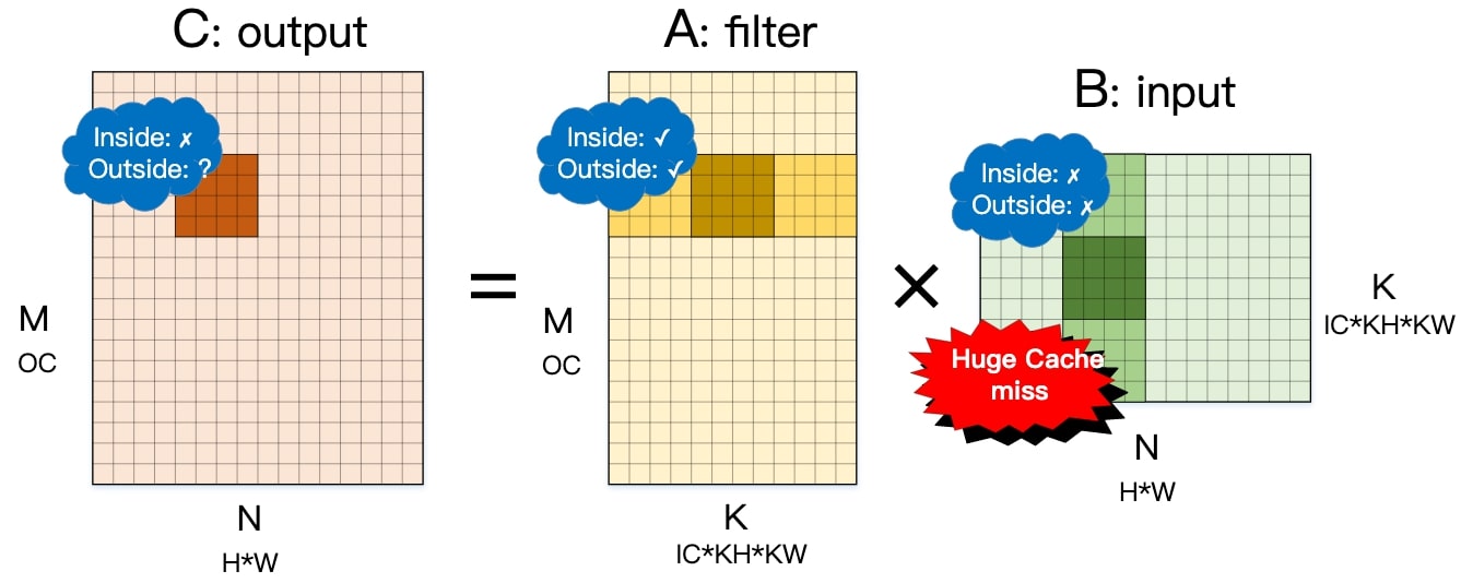 Figure 5: Analysis of Cache Behavior of NCHW Data Layout.
For input, the core loop of micro kernel gemm_8x8() loads eight vectors of length eight, dark green in Figure 5 as example. The address distance (\(H \times W\)) of neighboring vector is larger than 64 (cache line length) for most deep learning workloads, resulting 8 cache misses of 8 data loads. The 8 cache lines loaded from memory are not shared within a block step. Even worse, they are not shared across block steps, which is obvious. In this way, NCHW data layout leads to huge cache miss.
A straightforward optimization is packing input data to ease the cache miss issue. Nevertheless, QNNPACK enjoys smooth cache performance without transforming data layout.
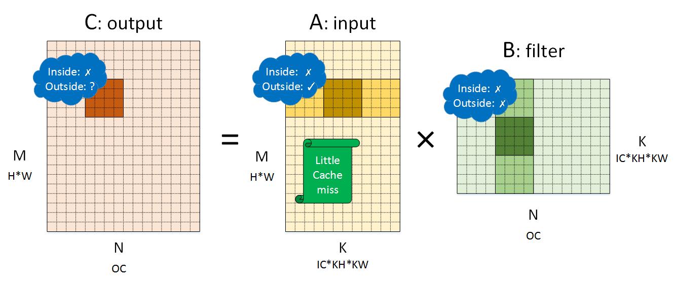 Figure 6: Analysis of Cache Behavior of NHWC Data Layout.
The matrix multiplication equivalent computation of NHWC pointwise convolution is as Figure 6. For input, neighboring block steps share data that loaded into same cache line. Therefore, cache miss can be significantly reduced in NHWC data layout.
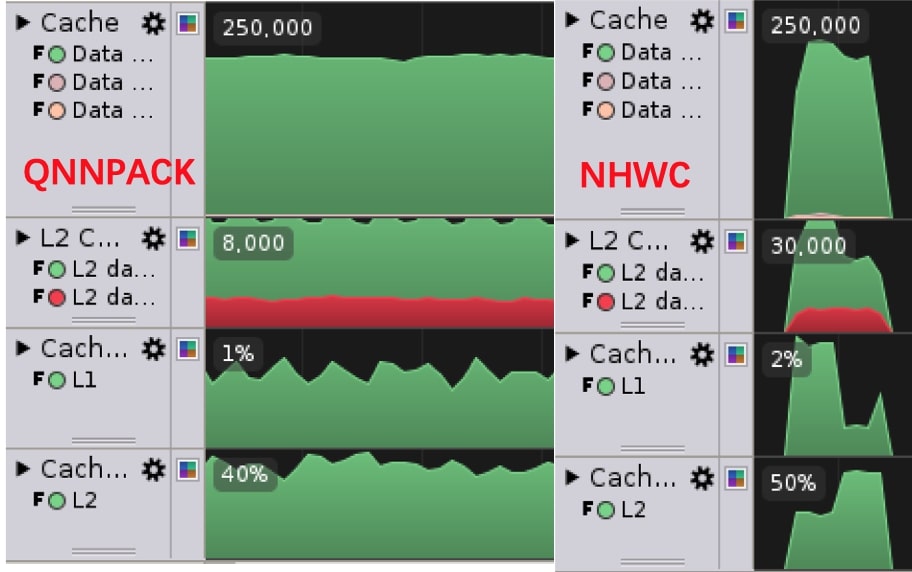 Figure 7: Cache Miss of QNNPACK and our NHWC Implementation.
Figure 7 shows that L1 cache miss rate has been reduced to 2% with new schedule which utilizes NHWC data layout. The performance improved significantly too.
After the investigation, we switched to NHWC data layout for potentially better performance.
Joint-tuning of AutoTVM and Tensorize
In practice, AutoTVM distinguishes TVM from many other engines because it is able to search good enough schedule for different networks and devices automatically.
However, tensorize schedules may encounter issues when integrating with AutoTVM. For example, micro kernel which computes an \(8 \times 8\) block is incompatible with workloads that cannot be divided by 8, which is the most case.
To leverage the power of AutoTVM, we refactored the schedules such that the AutoTVM generated configurations can pass to tensorized micro kernels to further to improve performance. The schedule templates of AutoTVM manage macro computation, and the tensorized kernel manages micro computation.
We also extended the micro kernel to support 64 scenarios of block size \(M \times N\) where \(M \le 8, N \le 8\). The enhanced schedule enables all kinds of workloads, and AutoTVM can select better micro kernel configurations regarding different devices. For example, \(8 \times 8\) block is better on AArch64, while \(4 \times 8\) or \(2 \times 8\) is better for Arm32 which holds less registers. Such observations have become experiences benefiting network architecture designs.
Depthwise Convolution Optimization
For depthwise convolution, we didn’t employ tensorize but leverage TVM schedule primitives.
The optimization firstly rewrote the schedule to eliminate data packing of original Spatial Pack design. In other words, the schedule computes depthwise convolution directly. This design improves performance by 10.1%.
For quantization computation, data needs to accumulated in int32 in case of overflow, and the multiplication is also in int32 format. However, if the input data type is int16, codegen can use ARM instruction smlal to perform the computation.
We also empolyed compute_at to adjust the compute and store, in which way to fix the trade off of between parall and compute locality. The technique improves 180% performance of the first depthwise convolution of our landing models.
Evaluation
The implementation has been evaluated on Raspberry Pi 3 Model B+ (with Ubuntu AArch64 installed) and compared with QNNPACK and TFLite.
The evaluation data is presented with: \(Benchmark\ Result = \frac{Lentency\ of\ Compared\ Engine}{Lentency\ of\ AliOS\ TVM}\)
Performance of Convolution
We extracted the convolution workloads of MobileNetV2, and compared with QNNPACK in Figure 8. QNNPACK is a high-performance kernel library that is optimized for mobile AI.
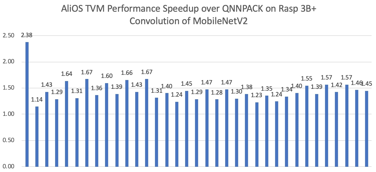 Figure 8: Quantization Inference Performance Compared with QNNPACK.
TVM is faster than QNNPACK for all MobileNetV2 convolution workloads. As QNNPACK is actually leading quantization inference performance on mobile devices, the optimization result is significant.
Performance of Depthwise Convolution
We extracted the depthwise convolution workloads of MobileNetV2, and compared with QNNPACK in Figure 9.
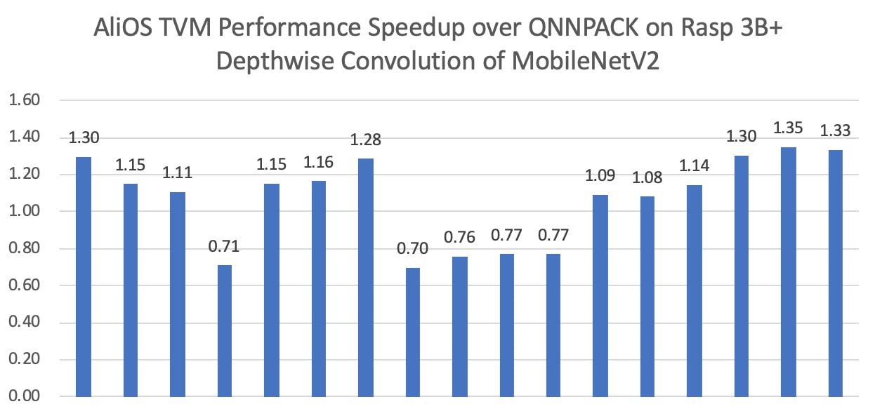 Figure 9: Quantization Inference Performance Compared with QNNPACK.
As we can see from the figure, TVM is faster than QNNPACK for most workloads. For other workloads that QNNPACK is faster, they take minor share of the overall latency.
Performance of End to End Networks
End to end network performance evaluation in comparison of TFLite is as Figure 10. TFLite is chosen because QNNPACK is a kernel library which can not run these networks directly.
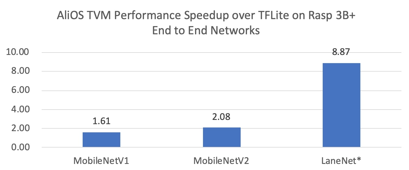 Figure 10: Quantization Inference Performance Compared with TFLite.
Figure 10 compares inference latency against TFLite of MobileNetV1, MobileNetV2 and LaneNet (a private landing model). For benchmarks models like MobileNetV2, TVM shows 2X improvement because TFLite has been optimized for them. When it comes to landing models which have rough workloads, TVM is much faster because it can adapt to the workloads and devices.
Conclusion
This artical summaries techniques utilized in convolution optimization for TVM. With AutoTVM empowered auto-tuning, carefully designed schedule algothrims and fine-grain computation manipulation may achieve impressive optimization results.
Reference