Preface

I had been planing to write a series articles on neural network quantization for a while. This Neural Network Quantization Introduction draws the skeleton.

Regarding the rapid evolution of deep learning in recent years, there has been plenty of metarils on quantiaztion. However, for most of these documents, authors rush into their works so fast that new comers can hardly understand even the baseline. This is of course not a good status in such a fast growing field.

My original plan was to discuss every aspects of quantization and try make them easy to understand. The theory, arithmetic, research and implementation may all be addressed. As titled, this article is the introduction which focus on background and theory. More will come but may not include the Neural Network Quantization keyword in their titles.

The series assume that readers are faimilar with Machine Learning, Neural Network and Deep Learning. If not, Andrew Ng’s Machine Learning course is a very good start. Google also provides tremendous materials which are TensorFlow based. If you are interested in more academy- or theory-style things, try Goodfellow’s Deep Learning book and Fei-Fei Li’s Convolutional Neural Networks for Visual Recognition (aka. cs231).

Lastly, why in English? Well, it seems impossible find translation of terminologies which meets a standard of 信雅达 for active researches like Neural Networks.

Introduction of Introduction

This section covers why introducing neural network quantization and abstracts some researches and industry solutions.

Why Quantization

Deep learning has been proven to be powerfull on tasks including image classification, objection detection, natural language processing and so on. Enormous applications are equipped with image (computer vision) related deep learning algorithms, Animoji for example. People use these applications without even aware the existence of such technology.

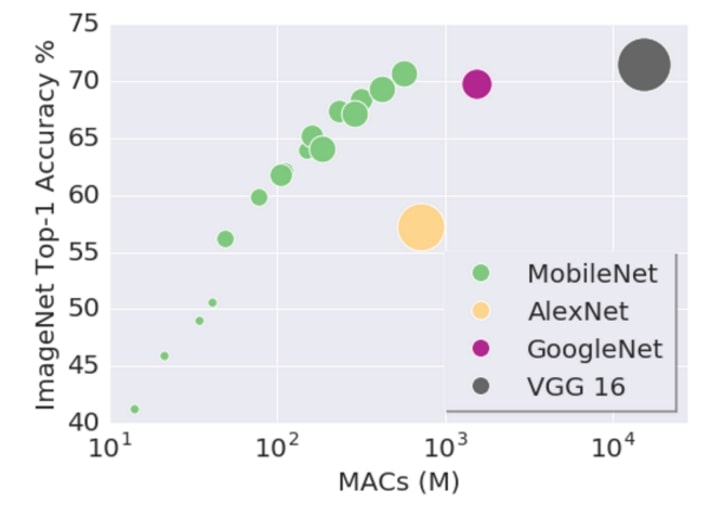Figure 1: Model MACs and Predicate Accuracy of Networks.

The deep learning algorithm (or model) improvements on ImageNet ever since AlexNet are related with model size somehow. In Figure 1 above, which is presented by Google researchers, the vertical is how good the network on is its task, the horizontal is how large (higher Multiply ACcumulate, larger model) the network is. AlexNet, GoogleNet and VGG together demenstrate that, if you have a large model, you are likely to get high accuracy. MobileNet is carefully designed such that it can have comparable accuracy with GoogleNet while still maintains a small model size. On the other hand, MobileNet itself of different size indicates that, maybe a good model design can help, but it’s still larger network, better score!

As we want more and more accurate predication, and as networks grows deeper and deeper, the memory size of network becomes a problem (Figure 2), especially on mobile devices. Typically, mobile phones are equipped with 4GB memory (as of early 2019), which is expected to be able to support multiple applications at one time. Models of large size make phones short of memory since they may take 1GB memory away if three or more models at one time which is usually the case.

The model size is not only a memory usage problem, it’s also a memory bandwidth problem. Weights of model is walked every time for each predication, and image related applications usually need to process data in real time, which means at least 30 FPS (Frame per Second). So, if deploying ResNet-50 to classify objects, which is relatively small, 3GB/s memory bandwidth is required for the model regardless other media processing. Memory, CPU and battery burn the device when network is runing. We cannot afford such a expensive effort to get a device a bit smarter.

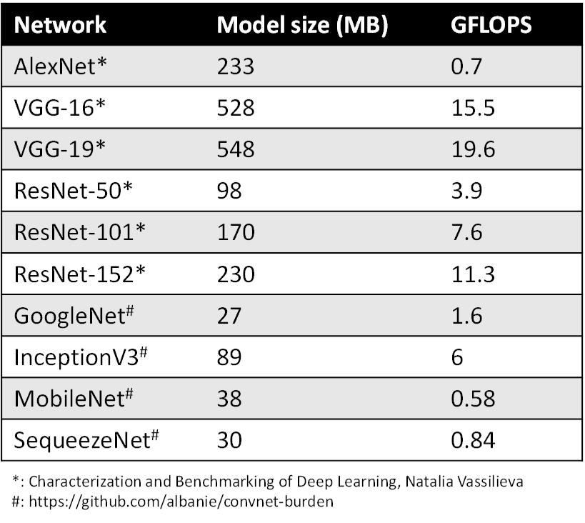Figure 2: Model Size and GFLOPS of Networks.

So efforts has been put to optimize the scheme of deep learning things. Researches basically lie in two aspects:

• Designing more effecient network architecture which maintains reasonable accuracy with relative smaller model size. MobileNet and SequeezeNet are such attempts.
• Reducing network size by means of compression, encoding and so on. Quantization is one of the most widely adopted compression methods.

These two aspects sometimes can co-work and achieve impressive results. For example, the quantized MobileNetV1 of TensorFlow is only 4.8MB, which is even smaller than most GIF. Therefore, such models can be easily deployed on any mobile platforms.

Quantization itself, conceptly, converts floating-point arithmetic of neural networks into fixed-point, and makes real time inference possible on mobile phones as well as benefits cloud applications.

Researches

Quantization has several other terminologies which could be similar in technique or concept.

Low precision could be the most generic concept. As normal precision uses FP32 (floating point of 32 bits which is single precision) to store model weights, low precision indicates numeric format such as FP16 (half precision floating point), INT8 (fixed point integer of 8 bits) and so on. There is a tend that low precision means INT8 these days.

Mixed precision utilizes both FP32 and FP16 in model. FP16 reduces half of the memory size (which is a good thing), but some parameters/operators have to be in FP32 format to maitain accuracy. Check Mixed-Precision Training of Deep Neural Networks if you are interested in this topic.

Quantization is basically INT8. Still, it has sub-categories depending on how many bits it takes to store one weight element. For example:

• Binary Neural Network: neural networks with binary weights and activations at run-time and when computing the parameters’ gradient at train-time.
• Ternary Weight Networks: neural networks with weights constrained to +1, 0 and -1.
• XNOR Network: the filters and the input to convolutional layers are binary. XNOR-Networks approximate convolutions using primarily binary operations.

Some other researches pay more attention to how to compress models rather that how many bits to store one element. Deep Compression is one of the most solid works, which assembles pruning, quantization and encoding to reduce the storage requirement by 35x (AlexNet) to 49x (VGG-19) without affecting their accuracy. The paper shows that 8 bit is required for quantized Convolution layer to avoid significant accuracy loss, while 4 bit is sufficent for Fully Connected layer, as Figure 3.

Figure 3: Weight bits and Network Accuracy in Deep Compression

Cheng Yu’s survey on model compression lists many works and categories them into parameter pruning and sharing, low-rank factorization and sparsity, transferred/compact convolution filters, and knowledge distillation.

Industry

Theory is one thing, practice is another. If a method is hard to generallize, significant extra enabling effort is required. Fancy researches are often of implementations so tricky or assumptions so strong that can hardly be introduced to generic software stacks.

Industry eventually chose the 8 bit quantization among the technologies described in Researches section. In 8 bit quantization, FP32 is replaced by INT8 during inference, while training is still FP32.

TensorRT, TensorFlow, PyTorch, MxNet and many other deep learning softwares have enabled (or are enabling) quantization. In general, solutions can be categoried according to the mechanism converting FP32 and INT8.

Some frameworks simply introduce Quantize and Dequantize layer which converts FP32 to INT8 and the reverse, when feeding to and fetching from Convolution/Fully Connected layer. In this case, the model itself and input/output are in FP32 format, as top half of Figure 4. Deep learning framework loads the model, rewrites network to insert Quantize and Dequantize layer, and converts weights to INT8 format.

Figure 4: Mixed FP32/INT8 and Pure INT8 Inference. Red color is FP32, green color is INT8 or quantization.

Some other frameworks convert the network into INT8 format as a whole, online or offline. Thus, there is no format translation during inference, as bottom half of Figure 4. This method needs to support quantization per operator, for the data flowing between operators is INT8. For the not-yet-supported ones, it may fallback to Quantize/Dequantize scheme. The remaining part of this article is based on this scheme.

As INT8 represents one number by only 25% bits of FP32, the policy that converts number between INT8 and FP32 is very important as it will impact predication accuracy significantly.

Quantization Arithmetic

Quantization process can be divided into two parts: converting model from FP32 to INT8, and inferencing with INT8. This section illustrates the arithmetic behind these two parts. Without understanding of the underlying arithmetic, you may usually get confused when considering details of quantization.

Fixed-point and Floating-point

Few people working on computer science have knowledge of how arithmetic operation is performed. As quantization bridges the fixed point and floating point, arihtmetic knowledge of them is a necessery prior one to understand related researches and solutions.

Fixed point and floating point are both representation of numbers. The difference is where the point, which divides the integer part and fractional part of a number, is placed. Fixed point reserves specific number of digits for both parts, while floating point reserves specific number of digits for significand and exponent respectively.

Figure 5: Format and example of fixed-point and floating-point.

Figure 5 gives the format and example of fixed-point and floating-point representations. For fixed-point, \(I\) denotes integer and \(F\) denotes fraction in \(IIIII.FFFFF\). For floating-point, the base is 2,10 and 16 for binary, decimal and hex format respectively. The digit examples of fixed-point and floating-point are the one-to-one same in Figure 5.

In the context of premitive data type of ISA (Instruction Set Architecture), fixed point is integer which doesn’t reserve fractional part, floating-point is in binary format. Generally speaking, fixed point is continuous since it is integer and the gap of two nearest representable numbers is 1. Floating point, on the other hand, the representation gap is determined by exponent. Thus, floating point has very wide value range (for 32 bits, max integer is \(2^{31}-1\) and max float is \((2 − 2^{−23}) × 2^{127}\)), and the closer the value is to 0, more accurate it can represent a real number. One observation is that, floating point has same number of values in different range determined by exponent as Figure 6. For exmple, the number of floating point values in \([1, 2)\) is same as \([0.5, 1)\), \([2, 4)\), \([4, 8)\) and so on.

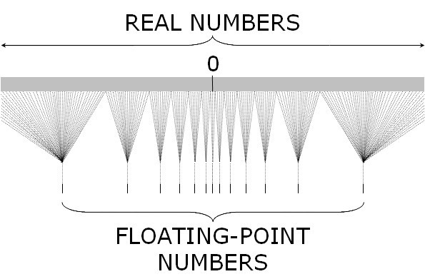Figure 6: Real numbers and floating point numbers.

Floating point operation can be composed by integer operations. In the early days, it is software which emulates floating-point arithmetic on fixed-point only hardware. Equations below show how floating-point multiplication is resolved into multiplication and addition of integer - the \(significand\) and \(exponent\). Addition is far more complex, we won’t go far in this part.

\(\begin{align} z &= x \times y \\ z_{significand} \times {base}^{z_{exponent}} &= (x_{significand} \times {base}^{x_{exponent}}) \times (y_{significand} \times {base}^{y_{exponent}}) \\ &= (x_{significand} \times y_{significand}) \times ({base}^{x_{exponent}} \times {base}^{y_{exponent}}) \\ &= (x_{significand} \times y_{significand}) \times {base}^{x_{exponent} + y_{exponent}} \end{align}\) Equation: Floating-point Mutiply.

In practice, after the integer multiplication of significand above, a rescaling operation is usually needed when the multiplication results in a number is too large for the representation, as Figure 7. Rescaling moves part of the significand result to exponent, and round the remained significand in a nearest rounding approach. The right half of Figure 7 is an example. Because some digits are abandoned, floating-point multiplication loses some information.

Figure 7: Significand part of floating-point multiplication.

Quantizing Floating-point

Neural networks are built of floating point arithmetic. As stated in Fixed-point and Floating-point, value ranges of FP32 and INT8 are \([ (2 − 2^{−23}) \times 2^{127}, (2^{23} - 2) \times 2^{127}]\) and \([-128, 127]\), while the value count approximate \(2^{32}\) and \(2^8\) respectively. Therefore, converting networks from FP32 to INT8 is not a trivial work like truncated casting of data types.

Fortunately, the value distribution of neural network weight is of small range, which is very close to 0. Figure 8 shows weight distribution of 10 layers (layers that have most value points) of MobileNetV1.

Figure 8: Weight distribution of 10 layers of MobileNetV1.

With such value range in \((-1, 1)\), quantizing floating point is mapping FP32 to INT8 using method like \(x_{float} = x_{scale} \times x_{quantized}\), where \(x_{float}\) denotes the FP32 weight, \(x_{quantized}\) denotes the quantized INT8 weight, and \(x_{scale}\) is the mapping fractor (scaling factor). Sometimes, we don’t want to map FP32 zero to INT8 zero, thus the equation is as Equation 5 and called uniform quantization in digital signal processing.

The unsigned integer is chosen in most cases, such that the INT8 value range is \([0, 255]\). The \(zero\_point\) is more meaningful in such scenario. In particular, quantizing float value is as Equation 6-9 below, and can be summarized in two steps:

1. Determining \(x_{scale}\) and \(x_{zero\_point}\) by finding min and max value in weight tensor.
2. Converting weight tensor from FP32 to INT8 per value.

Note that, rounding is needed in these steps when the floating-point operation result doesn’t equal to an integer. Considering mapping \([-1, 1]\) FP32 range to INT8 range \([0, 255]\). We have \(x_{scale} = \frac{2}{255}\), and \(x_{zero\_point} = 255 - \frac{255}{2} \approx 127\). Equations in this article are intended to be easy to understand, please refer to Quantization and Training of Neural Networks for Efficient Integer-Arithmetic-Only Inference if you are interested in more formal reasoning.

It’s obverious that there is error in quantization process. The error is inevitable just like the quantization in digital signal processing, where the quantization terminology comes from. Figure 10 shows the quantization and the error of digital signal processing.

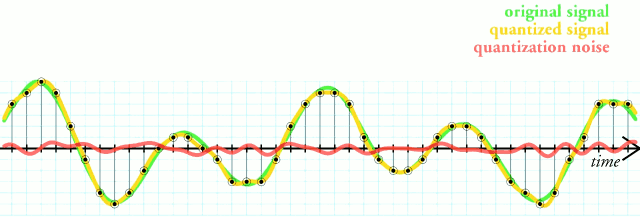Figure 9: Quantization and the error of digital signal processing.

Quantized Arithmetic

One essential thing of quantization to remeber is that, the quantized arithmetic represents non-quantized arithmetic, which means the INT8 computation in quantized neural networks is a reinterpretation of the FP32 computation of a normal neural networks.

The theory behind arithmetic representation is very similar with the floating-point multiplication (Equation 2-5) procedure illustrated in Fixed-point and Floating-point section.

Equation 10-16 below is the detail behind quantized multiplication \(x_{float} \cdot y_{float}\). \(Multiplier_{x,y,z}\) in Equation 15 denotes \(\frac{x_{scale} \cdot y_{scale}}{z_{scale}}\) of Equation 14. Since the scale factors of input \(x\), weight \(y\) and output \(z\) are all known for a given neural network, thus \(Multiplier_{x,y,z}\) can be pre-computed before network forwarding. Therefore operations in Equation 16 are in integer except the multiplication between \(Multiplier_{x,y,z}\) and \((x_{quantized} - x_{zero\_point}) \cdot (y_{quantized} - y_{zero\_point})\).

\(\begin{align} z_{float} & = x_{float} \cdot y_{float} \\ z_{scale} \cdot (z_{quantized} - z_{zero\_point}) & = (x_{scale} \cdot (x_{quantized} - x_{zero\_point})) \cdot (y_{scale} \cdot (y_{quantized} - y_{zero\_point})) \\ &= x_{scale} \cdot y_{scale} \cdot (x_{quantized} - x_{zero\_point}) \cdot (y_{quantized} - y_{zero\_point}) \\ z_{quantized} - z_{zero\_point} &= \frac{x_{scale} \cdot y_{scale}}{z_{scale}} \cdot (x_{quantized} - x_{zero\_point}) \cdot (y_{quantized} - y_{zero\_point}) \\ z_{quantized} &= \frac{x_{scale} \cdot y_{scale}}{z_{scale}} \cdot (x_{quantized} - x_{zero\_point}) \cdot (y_{quantized} - y_{zero\_point}) + z_{zero\_point} \\ Multiplier_{x,y,z} &= \frac{x_{scale} \cdot y_{scale}}{z_{scale}} \\ z_{quantized} &= Multiplier_{x,y,z} \cdot (x_{quantized} - x_{zero\_point}) \cdot (y_{quantized} - y_{zero\_point}) + z_{zero\_point} \\ \end{align}\) Equation: Quantized multiplication arithmetic.

For most scenarios where Equation 15 can apply, the \(quantized\) and \(zero\_point\) are INT8, the \(scale\) are FP32. Arithmetic operations between those two INT8 are INT16 or INT32 in practice, since INT8 can hardly hold the result of the operation. For example, let \(x_{quantized} = 20\) and \(x_{zero\_point} =50\), we have \((x_{quantized} - x_{zero\_point}) = -30\) which is out the INT8 value range \([0, 255]\).

A data type casting may covert the FP32 result of \(Multiplier_{x,y,z} \cdot (x_{quantized} - x_{zero\_point}) \cdot (y_{quantized} - y_{zero\_point})\) to INT32 or INT16. This result and \(z_{zero\_point}\) together gurrantee that the quantized result (mostly or very nearby if not) falls in INT8 value range \([0, 255]\).

Equation 17-26 are the quantized addition arithmetic. We won’t go into the detail since it is very similar to multiplication.

\(\begin{align} z_{float} & = x_{float} + y_{float} \\ z_{scale} \cdot (z_{quantized} - z_{zero\_point}) & = (x_{scale} \cdot (x_{quantized} - x_{zero\_point})) + (y_{scale} \cdot (y_{quantized} - y_{zero\_point})) \\ Multiplier_{x,y} &= 2 \cdot max(x_{scale}, y_{scale}) \\ z_{scale} \cdot (z_{quantized} - z_{zero\_point}) &= Multiplier_{x,y} \cdot \left( \frac{x_{scale}}{Multiplier_{x,y}} \cdot (x_{quantized} - x_{zero\_point}) + \frac{y_{scale}}{Multiplier_{x,y}} \cdot (y_{quantized} - y_{zero\_point}) \right) \\ Multiplier_{x} &= \frac{x_{scale}}{Multiplier_{x,y}}; Multiplier_{y} = \frac{y_{scale}}{Multiplier_{x,y}} \\ z_{scale} \cdot (z_{quantized} - z_{zero\_point}) &= Multiplier_{x,y} \cdot \left( Multiplier_{x} \cdot (x_{quantized} - x_{zero\_point}) + Multiplier_{y} \cdot (y_{quantized} - y_{zero\_point}) \right) \\ z_{quantized} - z_{zero\_point} &= \frac{Multiplier_{x,y}}{z_{scale}} \cdot \left( Multiplier_{x} \cdot (x_{quantized} - x_{zero\_point}) + Multiplier_{y} \cdot (y_{quantized} - y_{zero\_point}) \right) \\ Multiplier_{x,y,z} &= \frac{Multiplier_{x,y}}{z_{scale}} \\ z_{quantized} - z_{zero\_point} &= Multiplier_{x,y,z} \cdot \left( Multiplier_{x} \cdot (x_{quantized} - x_{zero\_point}) + Multiplier_{y} \cdot (y_{quantized} - y_{zero\_point}) \right) \\ z_{quantized} &= Multiplier_{x,y,z} \cdot \left( Multiplier_{x} \cdot (x_{quantized} - x_{zero\_point}) + Multiplier_{y} \cdot (y_{quantized} - y_{zero\_point}) \right) + z_{zero\_point} \end{align}\) Equation: Quantized addition arithmetic.

Besides multiplication and addition, there are many other arithemtic operations such as division, subtraction, exponentation and so on. There are particular methods, which can be decomposed into multiplication and addition, to represent these operations in quanzation regardless of whether it is complex or not. With theses methods the quantized neural network forwards and generates valid result just like the network it quantizes from.

Quantization Tweaking

This section moves attention to industry proposed trending solutions which handles practical problems when converting FP32 to INT8.

The Accuracy Problem

The method described in Quantizing Floating-point section is pretty straightforward. In the early development of a framework (or engine or whatever else you call it), that trivial approach is applied to make INT8 able to run. However, the predication accuracy of such INT8 quantized network usually drops significantly.

What happened? Though the value range of FP32 weight is narrow, the value points are huge. Taking the scaling example, \(2^{31}\) around (yes, basically half of the representables) FP32 values in \([-1, 1]\) are mapped into 256 INT8 values. Now consider two important rules discussed in Quantization Arithmetic section:

• The value density improves as floating-point values approach zero. The nearer a value is to zero, the more accurate it can be.
• The uniform quantization approach maps dynamic value density of floating-point to fixed-point of which the value density is constant.

So in the naive quantization approach, the floating-point values that near zero are less accuratly represented in fixed-point than the ones are not when quantizing. Consequently, the predicate result of quantized network is far less accurate when compared with the original network. This problem is inevitable for uniform quantization.

Equation 4 shows that the value mapping precision is singificantly impacted by \(x_{scale}\) which is derived from \(x_{float}^{min}\) and \(x_{float}^{max}\). And, weight value distribution such as Figure 8 shows that the number of value points near \(x_{float}^{min}\) and \(x_{float}^{max}\) are often ignorable. So, maybe the min and max of floating-point value can be tweaked?

Figure 10: Tweaking min/max when quantizing floating-point to fixed-point.

Tweaking min/max in Figure 10 means chosing a value range such that values in the range are more accurately quantized while values out the range are not (mapped to min/max of the fixed-point). For example, when chosing \(x_{float}^{min} = -0.9\) and \(x_{float}^{max} = 0.8\) from original value range \([-1, 1]\), values in \([-0.9, 0.8]\) are more accurately mapped into \([0, 255]\), while values in \([-1, -0.9]\) and \([0.8, 1]\) are mapped to \(0\) and \(255\) respectively.

Tweaking Approaches

The tweaking is yet another machine learning process which learns hyper parameter (min/max) of the quantization network with a target of good predicate accuracy. Different tweaking approaches have been proposed and can be categoried into Calibration (post-training quantization) and Quantization-aware Training according to when the tweaking happens.

TensorRT, MXNet and some other frameworks that are likely to be deployed in inference enviroment are equipped with calibration. Top half of Figure 11 is the process of calibration which works with pre-trained network regardless of how it is trained. Calibration often combines the min/max searching and quantization into one step. After calibration, the network is quantized and can be deployed.

Nvidia presented solid knowledge such as architecture and experiments on calibration. Check their slides of GTC2017 and blog.

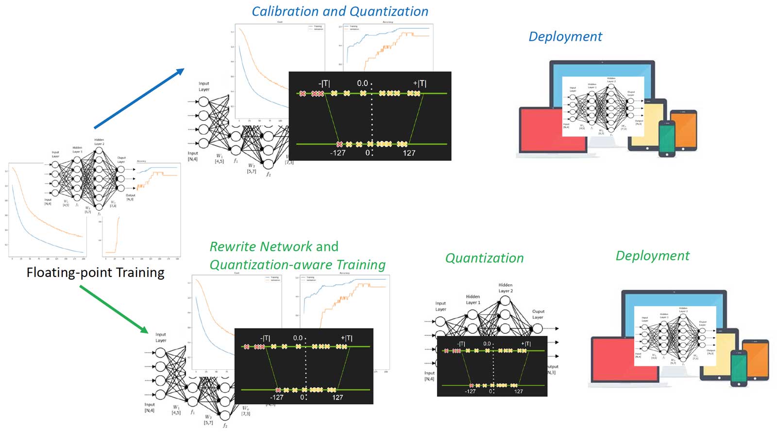Figure 11: Calibration and quantization-aware training process.

As calibration choses a training independent approach, TensorFlow inovates quantization-aware training which includes four steps:

1. Training models in floating-point with TensorFlow as usual.
2. Training models with tf.contrib.quantize which rewrites network to insert Fake-Quant nodes and train min/max.
3. Quantizing the network by TensorFlow Lite tools which reads the trained min/max of step 2.
4. Deploying the quantized network with TensorFlow Lite.

Step 2 is the so-called quantization-aware training of which the forwarding is simulated INT8 and backwarding is FP32. Figure 12 illustrates the idea. Figure 12 left half is the quantized network which receives INT8 inputs and weights and generates INT8 output. Right half of Figure 12 is the rewrited network, where Fake-Quant nodes (in pink) quantize FP32 tensors into INT8 (FP32 actually, the original FP32 was Quantize and Dequantize to simulate the quantization arithmetic) on-the-fly during training. The network forwarding of Step 2 above simulates the INT8 inference arithmetic.

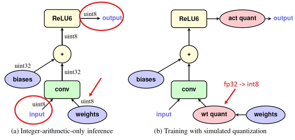Figure 12: Network node example of quantization-aware training.

Google revealed many details of quantization-aware training in Quantization and Training of Neural Networks for Efficient Integer-Arithmetic-Only Inference.

Summary

This ariticle introduces the background of neural network quantization, talks a lot on the underlying arithmetic of quantization, and lists some researches and industry solutions. These knowledge should be able to help people have a basic understanding of the quantization.

You may ask why quantization works (having a good enough predication accuracy) with regard to the information losing when converting FP32 to INT8? Well, there is no solid theory yet, but the intuition is that neural networks are over parameterized such that there is enough redundant information which can be safely reduced without significant accuracy drop. One evidence is that, for given quantization scheme, the accuracy gap between FP32 network and INT8 network is small for large networks, since the large networks are more over parameterized.

After this introduction, we will dive into detail things of quantization.

Reference

All the references have been listed in the Neural Network Quantization Resources.